Working manuscript — research draft for public review.
Ground-level viewers and surface screening in visual-impact assessment
Abstract
A surface-screened viewshed used in visual-impact assessment should preserve the viewer's standing elevation while representing intervening obstructions. Using a digital surface model for both roles can place a nominal ground viewer above vegetation or buildings. Removing tall-feature locations afterward leaves retained sightlines unchanged. We examine how viewer support affects modeled project visibility and whether height exclusion reproduces ground-supported screening within calculation and public-property domains. Primary guidance and published workflows establish the context; constructed scenes, landscape comparisons and supplemental parameter tests distinguish the geometric effect, local classification changes and aggregated property findings. In Groton, a strict six-foot height exclusion retains 133,286 of 785,321 receiver locations. Surface-supported and ground-supported classifications differ at 1,674 retained locations. Under nominal settings, however, zero-coded excluded surface-only results reproduce the paired model's visible indicator at all 2,761 queries within portions of two public properties. Their screened any-visible findings remain unchanged across twelve height/cutoff combinations, although pointwise equality does not. Only one of sixteen selected nominal disagreements preserves the complete disagreement criterion through all eight prescribed surface stresses; these diagnostics are not measured error bounds. Unchanged property classifications can coexist with local differences, while nominal local agreement does not establish general equivalence. Ground support and obstruction should be specified separately, and any masking substitute tested within the intended reporting domain. The comparisons establish computational effects, not observed visibility or the adequacy of an opaque surface beneath vegetation.
Keywords: viewshed; visual-impact assessment; digital surface model; observer elevation; landscape planning.
1. Introduction
A viewshed used to assess a proposed development should represent the people whose views may change. For a person standing on the ground, the model must place the eye above the ground while accounting for buildings, vegetation and terrain between that person and the project. When a viewshed uses one elevation raster for both endpoint support and obstruction, the raster choice can change the question being answered. A digital terrain model (DTM) supports the eye at ground plus eye height but omits above-ground screening. A digital surface model (DSM) includes that screening but supports the eye above the vegetation or roof represented at the same location.
Viewshed maps help analysts select viewpoints and direct field assessment (Cilliers et al., 2023; Sullivan, 2021). A terrain-only map can provide a deliberately broad envelope of potential visibility. A surface-screened map makes a more specific claim about where buildings and vegetation obstruct the project. When that map is used to represent ground-level views, raising the modeled viewer can counteract the screening the DSM was introduced to represent. The map remains one part of an assessment that also considers field observations, visual contrast and the sensitivity of the affected resource, but it must be clear whose view the calculation describes.
Cilliers et al. (2023) found that their constructed DSMs agreed more closely with field visibility classifications than their DTMs. Their line-of-sight procedure used DTM-based elevations to construct endpoint features. In a heritage-landscape assessment, Peng et al. (2026) placed road observers 1.7 m above a LiDAR DTM and evaluated screening with a separate representation of buildings and major vegetation. Ground referencing and surface screening therefore already have direct applications in visual-impact assessment. Reviewing landscape visibility research published from 2000 to 2019, Inglis et al. (2022) found that bare-earth models remained prevalent and that incomplete methods reporting limited reproducibility.
Separate ground and obstruction representations are established in the literature. Bartie et al. (2011) used terrain to position an observer and separate surface and vegetation information to evaluate visual exposure. PixScape (Sahraoui et al., 2018) supports ground-referenced observers with additional surface heights. Its inverse mode places observers throughout a raster domain with a separately configured target height, including applications to pylons and wind turbines (Vuidel et al., 2019, pp. 9–10, 35–37). Labib et al. (2021) likewise used separate terrain and surface data for ground-level viewers, although their target was visible greenness rather than a fixed project point.
The elevated-viewer problem is also established. Lock (2012) explained how DSM calculations can represent viewers on buildings or woodland and proposed using surface and bare-ground information to remove false positives. Perkins (2019) removes locations associated with tall surface features after a DSM viewshed calculation. Parent and Lei-Parent (2023) exclude forest and building locations in their comparison, using a different categorical rule. These post-calculation exclusions restrict the reported cells while leaving the sightlines unchanged at retained locations. Their adequacy for ground-level viewers therefore depends on which differing results the exclusion removes.
The locations used to represent an affected property also matter. Dong et al. (2024) address tree- and building-related false inclusion in onshore-wind viewsheds while considering property yards and nearby roads. Such applications connect the modeled surface to a defined set of viewing locations, rather than relying on visible-area totals alone.
A surface-screened assessment should preserve the standing elevation of the intended viewer while introducing the obstructions that may screen the project. Established paired-surface and explicit-endpoint methods can do this. Substituting a DSM for terrain, however, can change both the screening and the viewer, while subsequent height exclusion leaves the retained sightlines unchanged. We evaluate the consequences of preserving ground-viewer support at two levels: the screening calculated at individual locations and the visibility reported for mapped resources. Constructed scenes, landscape comparisons and independently mapped public properties connect this geometric distinction to the reporting domain: a workflow can differ across the map yet reproduce the screening of particular resources. Individual-location screening may inform viewpoint selection and field assessment even when a property's any-visible classification remains unchanged. Ground-supported sightlines against the represented surface provide the computational reference; observed visibility remains a separate question.
2. Ground support, obstruction and the reporting domain
2.1. A fixed project point and ground-level viewers
Let denote ground elevation and denote the absolute elevation of the obstruction surface at horizontal location . The two surfaces must share a vertical reference, and their sampled positions must be comparable. A layer containing object height above ground has a different meaning: if is such a layer, the obstruction elevation is . Treating height above ground as absolute elevation would change both the scene and the resulting visibility.
For a viewer at , eye height above the ground gives
Here, ground-level viewers stand on the bare terrain represented by G. An accessible bridge, deck or elevated walkway can support a viewer above that terrain and requires its actual standing elevation. The appropriate reference follows the intended viewer; a DTM is not a substitute for every walkable surface.
The project point has a fixed absolute elevation . For example, a point at a stated height above a project's ground elevation is converted to absolute elevation once, using the same ground reference in every scenario. Replacing the support raster must not inadvertently raise or lower the project as well as the viewer.
For the planar explanation, let run from zero at the viewer to one at the project, with horizontal position . The sightline is
The paired model compares the intervening obstruction elevations S(x(t)) with this line. A sampled obstruction above the line blocks visibility. The computational method must specify whether equality also blocks, where it samples the line, how it interpolates the surfaces, and how it treats the endpoint cells. Curvature and refraction require an additional, consistently applied geometry for long-distance analysis. These numerical choices determine how the physical model is evaluated.
2.2. The three surface choices
The comparison uses the same project point and viewer positions for three calculations (Table 1). Terrain-only visibility tests the ground-supported sightline against the DTM. Surface-only visibility tests a DSM-supported sightline against the DSM. The paired calculation uses the DTM to support the viewer and the DSM to represent intervening obstruction. It performs one line-of-sight test using the two elevation roles.
These roles do not require a particular number of raster inputs. An analyst can construct viewer and project endpoints with explicit three-dimensional elevations and evaluate their sightlines against an obstruction surface, as supported by ArcGIS Line Of Sight (Esri, n.d.). A DTM/DSM pair and explicit endpoints can express the same physical model, although their numerical results still depend on preparation and sampling.
Table 1. Elevation roles in the matched comparison. The absolute elevation of the project point is fixed across rows.
| Model | Viewer eye elevation | Obstruction elevation |
|---|---|---|
| Terrain only (A) | ||
| Surface only (B) | ||
| Ground and surface (C) |
The terrain-only and paired models differ in their obstruction representation. The surface-only and paired models differ in the viewer's elevation. This arrangement permits each mapped disagreement to be traced to one of those changes, provided that preparation, sampling and the reporting domain remain common.
The surface-supported sightline is . Writing , it is raised above the ground-supported sightline by
The shift is largest near the viewer and decreases towards the fixed project point. Even a small elevation difference at the viewer can therefore change a classification where the ground-supported sightline passes close to an obstruction.
The equations also clarify how to interpret visible-area comparisons. If the DSM is everywhere at or above the DTM along the same evaluated ray, adding it as the obstruction surface cannot increase visibility from unchanged ground-supported endpoints. If the DSM is at or above the DTM at the viewer, raising that endpoint while retaining the same obstructions cannot decrease visibility in the planar model. Terrain-only and surface-only results have no corresponding universal ordering: a surface-only substitution adds screening and raises the viewer at the same time. A larger or smaller surface-only viewshed cannot be attributed to screening alone.
These relations depend on the stated conditions. Independently produced rasters may contain locations where S is below G, and resampling or registration can change the elevations tested along a ray. Such cases require inspection of the sampled geometry. Raster names do not establish the inequalities.
2.3. Exclusion after the calculation
A post-calculation height mask retains a surface-only result where the surface-ground difference is below a threshold :
We implement Perkins's (2019) six-foot-or-more exclusion with m, using international feet and excluding equality. This cutoff is distinct from the viewer's eye height.
At a retained location with , Equation 3 still applies. The mask has not changed the eye elevation or the clearances along the sightline. It can remove all differing cells in a particular scene, but it cannot guarantee a ground-supported result for the cells that remain. Testing this residual difference requires comparing the two calculations within the same retained domain, rather than comparing their total visible areas after different exclusions.
This explanation uses the same surface functions at the same viewer position to define both the eye displacement and the height mask. An implementation may instead resample the endpoint elevations and mask differently. In that case, the eye displacement and the masking value must be reported separately; agreement in their source raster names does not establish agreement in the elevations actually used.
The cutoff's relationship to eye height also matters. With common endpoint sampling, a cutoff above eye height places every height-excluded ground eye below the opaque DSM. An evaluator that tests the viewer's own location blocks it there. Assigning zero to the excluded surface-only results can therefore agree with the paired calculation at those locations, even though exclusion and evaluated blockage have different meanings. Supplementary methods state the equality and validity conditions.
Exclusion can be appropriate when it represents the population whose views are under assessment. Building interiors may lie outside a study of outdoor public viewpoints. Surface height, however, is an imperfect substitute for that population: a forested raster cell can contain a public path, an open understory or dense vegetation. The analysis should identify the receiver domain independently where evidence permits. A location excluded by a reporting rule should remain distinguishable from one whose sightline was evaluated and blocked.
 Open figure at full size
2.4. What the surface represents
A DSM assigns a single upper elevation to each cell. Used as an opaque obstruction envelope, it cannot describe an opening below a tree crown or an elevated structure. Cimburova and Blumentrath (2022) identified exposure-model outliers where photographs represented views beneath tree canopies but the modeled viewing positions were on the canopy surface. Separating ground support fixes the elevation from which a view is tested; it does not reconstruct those openings. Bartie et al. (2011) addressed vegetation structure and permeability explicitly, while Inglis et al. (2022) identified the limitations of single-height surface representations more broadly.
The endpoint convention is part of this physical specification. A nominal ground viewer beneath the DSM can represent an impossible position inside a solid structure, an accessible position beneath a canopy, or a cell whose upper elevation reflects an adjacent object. Excluding the receiver cell from intersection tests, testing a point at its centre and treating the entire cell as occupied are different assumptions. A two-raster interface alone does not resolve them. The present comparison includes the viewer-end obstruction sample, so a ground eye below its opaque surface is blocked locally.
3. Assessment guidance and documented practice
We examined primary guidance and documented workflows from New York environmental review and U.S. offshore wind. The comparison records endpoint references, obstruction representation, viewer heights, exclusion rules and the use of visibility outputs in field review. This targeted source selection identifies methodological differences without estimating their prevalence across the profession.
3.1. New York visual assessment
New York's DEC visual policy, DEP-00-2, addresses assessment under the State Environmental Quality Review Act, Environmental Conservation Law Article 8. It prefers viewshed analysis while accepting line-of-sight profiles and verification appropriate to the project and affected resource. Its glossary defines the profile's endpoints as the observer's eye elevation and an elevation of the project component (New York State Department of Environmental Conservation [NYSDEC], 2019, §VI.C and glossary). Appendix A illustrates vegetation added at appropriate locations and heights above a terrain profile. The conceptual separation of a viewer's position and intervening screening is therefore present in the guidance.
DEP-00-2 leaves the raster algorithm unspecified. It directs DEC staff in the designated SEQR roles and is advisory for other lead or involved agencies.
Public Service Law Article VIII establishes a separate energy-siting framework. The current renewable-energy provisions, effective 9 March 2026, require viewshed mapping and confirmatory visual-assessment fieldwork. Section 1101-2.8 requires mapping that accounts for topography and vegetation, line-of-sight profiles for resources of statewide concern within the study area, and a description of the software, baseline information and data sources. It also connects mapped visibility to the selection of viewpoints and viewer groups (New York State Department of Public Service [NYSDPS], 2026). These clauses specify relevant landscape features and assessment tasks without prescribing how separate ground and surface rasters enter a sightline calculation.
3.2. Offshore-wind guidance
BOEM's 2021 methodology distinguishes a terrain-based zone of theoretical visibility from a surface-screened assessment. It treats terrain-only visibility as generally overestimating visibility where buildings or vegetation screen the project and prefers a surface elevation model, verified through field surveys, for impact assessment and viewpoint selection (Sullivan, 2021, §5.4 and Appendix A.1.1). Thus, its recommendation already extends beyond a bare-earth viewshed.
Appendix A.1.2 specifies a 1.8-m viewer height and accurate viewpoint elevations, including additional elevation for deliberately elevated viewpoints. It also calls for earth curvature and atmospheric refraction. Appendix A.1.3 calls for documentation of procedures, parameters, data and software. An implementation for this purpose must explain how a surface-screened calculation preserves the intended viewpoint elevation across the assessment domain. The guidance does not supply a paired-raster algorithm, and its preference for an obstruction-bearing surface should not be read as a direction to place viewers on that surface.
3.3. Surface preparation, height masks and endpoint references
The Atlantic Shores visual-impact assessment documents one project workflow. Its methodology uses a 3-m DSM as the ArcGIS calculation surface and a six-foot viewer height, then sets visibility to zero where the surface exceeds bare ground by at least six feet (Environmental Design & Research [EDR], 2023, §2.2, pp. 59–60). Before calculation, it also replaces surface elevations with bare earth in transmission corridors and within 50 feet of road centre lines to remove modeled screening attributed to utility lines. The workflow therefore combines changes to the obstruction surface with a subsequent restriction on reported locations.
Corridor replacement changes intervening screening and can also make surface and ground elevations equal at road viewers, eliminating their endpoint displacement. Post-calculation exclusion instead removes completed results. Its residual effect can be tested by comparing ground-supported and surface-supported sightlines at the retained locations while keeping the obstruction surface unchanged.
The New York Bight assessment uses a related procedure (Hunt et al., 2024, §4.1, pp. 30–31). It runs separate ArcGIS Pro Visibility analyses on terrain and surface models, then filters the surface-model results using the difference between those rasters. Its stated retained threshold is at or below 5.5 feet, reported as 1.7 m. This differs from both the six-foot exclusion in Perkins and the assessment's stated calculation eye height of 5.25 feet, reported as 1.6 m. The resulting area of potential visual impact informs viewpoint selection and field review. These details show why naming both a DTM and a DSM in a report does not establish that they supplied separate roles within one calculation.
The Vineyard Mid-Atlantic assessment specifies Global Mapper Pro 25.0 and viewers 1.8 m above existing grade, but does not identify the supporting ground-layer selection or loaded-layer order in its methods (Saratoga Associates, 2024, §3.2.1, pp. 20–21). The reported information therefore leaves the endpoint and obstruction assignments unresolved.
Global Mapper Desktop documents a ground-reference layer selector separately from the loaded elevations used to assess obstructions. The reviewed raster-output interfaces in ArcGIS, GDAL and GRASS, including QGIS's GDAL provider, instead expose one elevation surface per operation (Supplementary Table S3). These interface differences help explain how a common request for ground-level screening can lead to different elevation assignments. They do not establish which assignment a published assessment used or exclude explicit-endpoint alternatives in those platforms.
4. Comparison design
4.1. A constructed sightline and an agreeing control
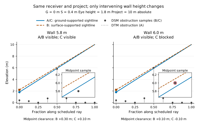
Two nine-sample constructed scenes use level ground at zero elevation, a fixed project elevation of 10 m, eye height 1.8 m and surface support 0.4 m above ground. Only the midpoint obstruction changes: 5.8 m in the agreeing control and 6.0 m in the second scene. Both eye positions are above the local surface, and the viewer passes the six-foot screen in both scenes. Equality is clear; curvature and refraction are omitted. The complete trace verifies the expected classifications, agreement between scalar and raster evaluations, and an intervening first blocker. Figure 1 and supplementary methods give the geometry and numerical tolerance.
4.2. Computational checks and their scope
The toolbox and standalone backend share an implementation; their agreement checks the ArcGIS entry point and input interpretation. Constructed scenes provide explicit geometric expectations. Native Global Mapper comparisons qualify correspondence only for the tested software configurations. Supplementary methods distinguish these checks from independent algorithm or field validation and identify the retained verification records.
4.3. Landscape data and study domains
The landscape comparison uses available telecommunications-project elevation data from Groton, Connecticut, and South Salem, New York. These cases permit controlled comparisons within existing terrain and surface representations. They were not selected as a representative sample of assessment practice, and differences between them cannot be attributed to landscape character alone because their preparation histories differ. Each comparison uses a nominal 1,000-m radius, 2-m output spacing and a 1.8-m eye height. These are study settings, not a reconstruction of the original assessments. The project is represented by one fixed point; the experiment does not model the visible extent of an entire structure or wind farm.
The Groton rasters were prepared in Global Mapper 25.1 from 16 tiles of the Connecticut 2016 Block 2 LiDAR collection. The collection metadata identify acquisition between 19 March and 13 April 2016, NAD83(2011) Connecticut State Plane coordinates and NAVD88 heights referenced through Geoid12B, originally in US survey feet (State of Connecticut, 2016). The 2-m DTM uses class-2 ground returns and a triangulated irregular network. The DSM uses maximum elevation per bin, excludes noise classes 7 and 18, and was generated without gap filling. The retained grids use metre elevations and EPSG:26956; their generic NAD83 CRS label does not resolve how the preparation handled the source's datum realization. The project height is approximately 53.34 m above the DTM, converted once to a common absolute elevation. The computational record retains the exact converted value.
The secondary South Salem comparison uses metric exports of a legacy DTM/DSM pair whose original vertical units, datum and construction history remain unresolved. It tests computational differences within that supplied pair, under the retained unit interpretation, rather than independently confirming a physical landscape effect. Supplementary methods document its inputs and limitations.
For both cases, the study inputs are integer-window crops of the retained rasters, with unchanged cell values. File hashes identify those inputs. Preparation and receiver sampling follow Section 4.4. Groton's independently selected receptor domain uses the town's Open Space layer, filtered by its public-access attribute (Town of Groton, n.d.). The portion of the domain within the study radius includes Copp Family Park and Great Brook Park. These property boundaries define locations to report; they do not establish suitable standing positions throughout either park. The municipal layer was retrieved in October 2026 and has no verified edition date. Its combination with the older elevation data is not a reconstruction of observed views at a single date.
4.4. Sampling controls in the landscape comparison
The landscape experiment separates a change in elevation roles from a change in how elevations are sampled. Ground support, surface support and the height-screen difference are evaluated at the same receiver query using the same prepared-grid sampler. The surface-only and paired calculations share the obstruction samples; the terrain-only and paired calculations share the ground-supported eye. Missing DSM cells use the prepared DTM as a fallback. Valid surface elevations below the ground raster are retained rather than raised to ground level. Here, S denotes that resolved obstruction surface, not the pointwise maximum of both rasters. The study runner changes receiver-support and height-screen sampling for this comparison; these are scientific controls rather than unchanged executions of the toolbox's ordinary preparation workflow. Toolbox qualification and native Global Mapper agreement are evaluated separately.
All three models share the same discrete ray schedule and fixed absolute project elevation. The scheduled target and receiver queries can differ from the requested project coordinate and output-cell centres; the supplementary methods identify those mappings. The radius domain follows output-cell centres, whereas property membership follows the actual receiver queries. Profiles use normalized sample position. The comparisons establish effects within this common discretization rather than validate continuous sightlines.
Curvature/refraction and Fresnel corrections are disabled. A valid sample blocks a ray only when its obstruction elevation is strictly above the sightline; equality is clear. A ray without an earlier blocker is invalid when missing samples exceed the integer floor of one-tenth of its scheduled sample count. These settings are common to the three models and do not reproduce the long-distance settings called for in offshore-wind guidance.
4.5. Comparing classifications and reporting exclusions
The landscape comparison distinguishes visibility at individual receiver locations from visibility aggregated over a public resource. For each pair of models, the pointwise comparison has four outcomes: both visible, both blocked, or either model visible while the other is blocked. Locations lacking a valid result in either model remain outside that pair's denominator and are reported separately. A valid surface-only and paired comparison does not require a valid terrain-only result.
The height exclusion is applied to the same receiver locations in both models. Results are reported before exclusion and within the common retained set, using the strict six-foot threshold in Section 2.3. The retained comparison is further separated by the sampled surface-ground difference: negative, zero, positive but below eye height, and at or above eye height. This distinguishes retained locations where the ground-supported eye is above the local DSM from those where it is at or below that envelope. Negative differences are preserved rather than changed to zero. Counts of excluded locations and unavailable elevations accompany the visibility counts, so agreement among retained locations cannot stand for agreement across the original viewer domain.
Public-resource boundaries define a reporting domain independently of the calculated visibility. Membership is evaluated at the coordinates where the model samples receiver support. A property's public-access designation does not establish that every enclosed raster location is accessible or suitable for standing; a mapped route provides a more specific receptor association where its source supports that interpretation. Counts of raster locations therefore describe the model's samples, not numbers of people. They also do not measure route length without an explicit spatial weighting rule.
Resource aggregation begins with the locations selected by geometry and the radius domain, before invalid model results are removed. An any-visible rule identifies potential visibility if at least one location known to be eligible has a valid visible result. Otherwise, a no-visible finding requires valid blocked results at every included location and no unresolved eligibility. After height screening, only locations known to be retained can establish visibility; unavailable mask values remain unresolved. Missing results therefore remain distinguishable from a resource with no samples in the radius domain or with every sample removed by the height screen. This aggregation is calculated both before and after the common exclusion. A resource can retain its potential-visibility classification despite changes at individual locations; conversely, agreement after exclusion can arise because the screen removed the locations at which the models differed.
4.6. Supplemental parameter and surface tests
After inspecting the nominal results, we conducted two supplemental tests. The property comparison retained all 2,761 original queries and crossed four eye heights (1.6, 1.6002, 1.8 and 1.8288 m) with three strict surface-ground cutoffs (1.6764, 1.7 and 1.8288 m). Each height was evaluated once; the cutoffs reused those classifications. Nominal support and classification checks passed. The combinations test parameter dependence rather than reconstruct complete historical assessments.
A separate diagnostic panel used nominal Groton settings. Sixteen retained surface-visible/ground-blocked locations with ground eyes above the local surface and intervening first blockers were selected, four from each rank quartile of complete-schedule clearance margin. Eight agreeing-visible and eight agreeing-blocked controls completed the panel. IDs were frozen after the property height passes but before perturbation outcomes. Exact zero-shift replay preceded eight stresses: separate ±0.10-m changes to prepared ground and resolved-surface fields, and shared 1-m translations east, west, north and south. Changed fields supplied support, obstruction and exclusion consistently; receiver positions, ray schedules and project elevation stayed fixed. The supplement specifies selection and sampling. These tests cover the property cohort and selected panel respectively, not full-landscape reruns under every variant. The imposed changes are hypothetical diagnostics, not measured error bounds.
5. Results
5.1. Height exclusion leaves the retained sightline unchanged
With the 5.8-m midpoint obstruction, all three models classify the sightline as visible. At 6.0 m, the paired model blocks while the surface-only model remains visible; their clearances are approximately -0.1 and +0.1 m. Terrain-only visibility omits the obstruction. The mask retains the viewer in both scenes. This establishes possible retained disagreement with clear viewer endpoints, while the agreeing control shows that endpoint displacement need not change a classification.
5.2. Residual differences across the Groton calculation domain
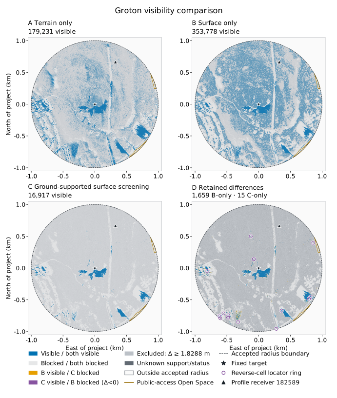
The complete Groton calculation includes 785,321 receiver locations, all with valid classifications in the three models. Terrain-only visibility identifies 179,231 visible locations, surface-only visibility 353,778, and ground-supported surface screening 16,917 (Table 2). The surface-only substitution therefore increases total visibility relative to the terrain-only calculation in this case, despite adding buildings and vegetation to the obstruction representation. Its simultaneous change in viewer elevation prevents interpreting that comparison as the effect of screening alone.
With common obstruction samples, surface support identifies more visible locations than ground support, with only 15 reverse disagreements. Supplementary Table S2 gives the joint classifications, including the terrain comparison; subtracting visible totals would conceal reverse differences.
The strict six-foot screen retains 133,286 locations. Within that set, the models disagree at 1,674 locations: 1,659 are visible only with surface support and 15 only with ground support. The former differences occur where the sampled surface elevation exceeds ground elevation; all 15 reverse differences occur among the 7,291 retained locations where the surface elevation is lower. No receiver has exactly equal sampled ground and surface elevations. The reverse differences therefore do not violate the conditional relation in Section 2.2, which requires the surface-supported eye to be at least as high as the ground-supported eye.
The first blocking sample separates two groups of retained positive differences. Among 125,355 locations with a positive surface-ground difference below eye height, 1,576 are visible with surface support but blocked by an intervening sample with ground support. The viewer's own obstruction sample does not cause these blockages. Another 640 retained locations have a surface-ground difference at or above the stored eye height and below the six-foot cutoff. Of these, 83 are visible only with surface support, and their ground-supported rays are blocked at the viewer sample. The other 557 are blocked in both models. Most retained directional differences therefore concern intervening screening; the smaller group is already blocked at the viewer under the opaque-surface assumption. Its first blockage does not establish that the remainder of the ray is clear.
All 652,035 height-excluded locations are blocked in the ground-supported model. Exclusion removes 335,217 surface-supported visible results, while the remaining 316,818 excluded locations were already blocked in both models. The residual disagreement concerns retained sightlines. Its occurrence across the wider calculation domain does not establish a change at an assessed public resource.
Table 2. Visible receiver locations under the three elevation assignments in Groton. The project elevation, receiver queries and sample schedule remain fixed. The retained column applies the same strict six-foot height rule to every model for this comparison; it does not imply that terrain-only screening ordinarily uses that rule.
| Model | All 785,321 locations | Common retained set: 133,286 |
|---|---|---|
| Terrain only | 179,231 | 41,747 |
| Surface only | 353,778 | 18,561 |
| Ground and surface | 16,917 | 16,917 |
 Open figure at full size
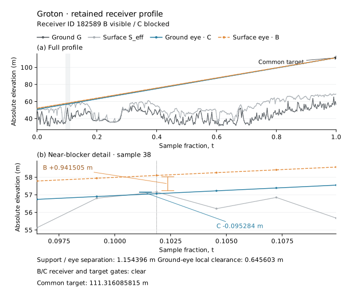
The retained profile in Figure 3 provides a landscape example of the intervening-blockage mechanism. Its surface support is 1.154 m above ground, below both eye height and the height cutoff. Both endpoint samples are clear. At sample 38, the surface-supported line clears the obstruction by 0.942 m, whereas the ground-supported line falls 0.095 m below it.
 Open figure at full size
5.3. Agreement after screening in the Groton property domain
The independently selected Groton property domain contains 2,761 receiver queries within the study radius: 1,536 in Copp Family Park and 1,225 in Great Brook Park. All have valid classifications and known support values. Before height exclusion, 1,112 locations are visible only with surface support, with no reverse disagreement (Table 3).
The strict six-foot screen removes 2,241 locations and retains 520. Every retained classification agrees: ten locations are visible in both models and 510 are blocked in both. Assigning zero to the excluded surface-only results, as in the tested post-calculation workflow, also produces exact binary agreement with the unmasked ground-and-surface result across all 2,761 locations: ten visible and 2,751 not visible. The exclusion mask remains separate so that this agreement does not erase the distinction between an excluded result and an evaluated blockage.
Table 3. Surface-supported and ground-supported classifications in Groton's public-property domain. Both calculations use the same obstruction samples. The reporting domain comprises receiver queries in the mapped property polygons within the nominal study radius. Excluded locations remain separately identified.
| Classification pair | Before height exclusion | Common retained set |
|---|---|---|
| Both visible | 10 | 10 |
| Surface-supported visible; ground-supported blocked | 1,112 | 0 |
| Surface-supported blocked; ground-supported visible | 0 | 0 |
| Both blocked | 1,639 | 510 |
| Valid comparison locations | 2,761 | 520 |
| Excluded by the height rule | 0 | 2,241 |
After the common screen, 482 locations remain in the Copp polygon and 38 in the Great Brook polygon. Both models classify the retained Copp locations as blocked and identify potential visibility at Great Brook under the any-visible rule. The viewer-support choice therefore does not change the post-screen resource classification for these two polygons. These findings concern the sampled portions within the study radius, rather than visibility throughout either park or verified standing positions along its paths.
5.4. Parameter dependence and selected surface stresses
Property screening remained unchanged throughout all twelve height/cutoff combinations: Copp had no screened visible query, while Great Brook had at least one under both models. Pointwise equality was parameter-specific (Supplementary Table S4). At the two lower eye heights, two or three retained queries were visible only with surface support. At the two higher heights, retained classifications agreed, but the two smaller cutoffs excluded one location visible in the unmasked paired model. A mask can therefore lose a paired-visible location even where every retained classification agrees. No support or classification was unavailable.
Among the sixteen selected disagreements, 13–15 persisted under each vertical stress and three or four under each translation. Only one location satisfied the complete retained, above-local-surface, surface-visible/ground-blocked and intervening-blocker criterion in all eight variants. This is a selected-case finding, not a landscape-wide robustness rate. All agreeing controls preserved their classifications under vertical stresses. East and north translations each changed one agreeing-visible control to surface-visible/ground-blocked; agreeing-blocked controls remained blocked in both models. Eligibility sometimes changed despite unchanged classifications.
5.5. Additional comparison within the legacy South Salem pair
Within the legacy South Salem pair, 354 retained locations are visible only with surface support: 332 first blockages occur at intervening samples and 22 at the viewer sample. No reverse disagreement occurs. These computational patterns resemble Groton's, but unresolved source metadata prevent a corresponding physical inference. Supplementary Table S1 gives the denominators and model totals.
6. Discussion
6.1. Viewer elevation and conditional agreement
At 1,576 retained Groton locations, the ground-supported eye is above the local surface, yet an intervening sample blocks its sightline while the surface-supported calculation remains visible. The viewer-support assignment therefore changes represented screening beyond the locations removed as rooftop or canopy viewers. This effect is distinct from the local blockage of an eye below the DSM envelope.
The Groton comparison separates disagreement across a map from agreement within a reporting domain. The height mask leaves differing retained sightlines across the map, yet reproduces every paired-model visible indicator in the two property subsets under the nominal settings. Agreement there supports a computational substitution for that result; it does not show that the sightlines or modeled viewer elevations are identical.
The supplemental property tests preserve the same resource classifications while changing pointwise agreement. This separates reproduction of a declared resource screen from reproduction of every sightline. It also shows why a result established under one height and cutoff should not silently carry over to other settings.
6.2. Implications for assessment practice
When a workflow is presented as a substitute for ground-supported surface screening, its adequacy should be assessed against the intended use. Matching any-visible resource classifications establishes agreement for that aggregate screen, but does not by itself establish agreement about where the project is modeled as visible. The nominal property subsets agree pointwise; lower-eye-height tests show local differences despite unchanged resource categories. Such differences could matter for viewpoint selection or local screening where the sampled queries represent relevant viewers. These uses do not require the assessment boundary or receptor inventory to change. A deliberately broader preliminary screen has a different purpose and should be identified as such.
A screened ground-viewer calculation should preserve the intended eye elevation when introducing surface obstructions. The reviewed guidance identifies viewpoint elevations and screening separately; implementation must preserve that distinction. Reporting a six-foot eye height without identifying its supporting surface leaves the viewer's actual elevation unresolved. Reporting both terrain and surface datasets does not establish that they supplied separate roles. A methods account should identify the endpoint references, obstruction representation and any changes made before calculation; it should then describe subsequent exclusions and how point results are aggregated into resource screening. This information lets a reviewer distinguish an intentional terrain-only envelope, a ground-supported screened map and a surface-supported map whose exclusions have been tested for equivalence.
6.3. Limits of the represented view
A correct ground reference is necessary for the declared ground viewer, but it does not establish that the obstruction model describes the view a person would experience. An opaque DSM can block a viewer beneath a tree crown even where a real understory view exists. A height mask can remove that same location for a different reason. Neither result establishes whether a visitor can stand there or see the project. Property boundaries associate the calculations with public resources; they do not resolve that physical or access question. Field observations could establish visibility and standing conditions at particular locations; a scene representing openings could test how the opaque-envelope assumption affects modeled visibility.
Elevation error and obstruction geometry can change a viewshed independently of the viewer's support elevation (Fisher, 1991; Sander & Manson, 2007). The selected diagnostic disagreements are particularly sensitive to imposed surface translations. Loss of their full persistence criterion can involve changed eligibility or local occupancy as well as changed visibility. That sensitivity limits claims about stable affected locations without negating the exact endpoint-displacement mechanism. The prescribed increments provide no measured error bounds, probabilities or field validation, and do not resolve the rasters' datum and source limitations.
The landscape cases and settings also bound the interpretation. The primary applied comparison uses one available project landscape and a limited portion of two public-property polygons. The legacy South Salem pair supplies a computational comparison with unresolved source metadata. The discrete sampling and fixed-point target permit controlled contrasts between elevation roles, but do not validate a continuous sightline, the visual prominence of a whole structure, or a long-distance offshore-wind viewshed. The offshore assessments motivate the parameter and workflow questions; their geometry and field conditions are not reproduced here.
7. Conclusion
Surface screening should be evaluated from the standing elevation of the viewer whose view is under assessment. Separate ground and obstruction representations can preserve that specification, as can explicit three-dimensional endpoints. A surface-supported calculation followed by height exclusion can reproduce resource screening without generally correcting the retained sightlines. In Groton, the two properties retain the same screened classifications across the tested parameter combinations, while pointwise agreement depends on settings and selected map disagreements respond to imposed surface changes. Local screening can remain relevant to viewpoint selection and field assessment when resource categories remain unchanged. Practitioners should state the support assigned to viewers, the obstructions tested and the domain in which a substitute workflow has been shown to agree. Evidence about standing conditions and obstruction openings remains necessary to interpret either calculation as a person's view.
Code and data availability
The supported ArcGIS Pro toolbox (Modern Viewshed Tools 0.1.0), installation instructions and synthetic examples are available from the toolbox page. The maintained code requires repository access. The retained study revision remains identified separately from later toolbox-interface updates and also requires repository access. The public download contains the operational toolbox and synthetic inputs. Reproducing the landscape analyses additionally requires the retained controlled-study runner and original raster inputs, which are not included. The supplementary methods document the computational record and input-provenance limitations.
References
Bartie, P., Reitsma, F., Kingham, S., & Mills, S. (2011). Incorporating vegetation into visual exposure modelling in urban environments. International Journal of Geographical Information Science, 25(5), 851–868. https://doi.org/10.1080/13658816.2010.512273
Cilliers, D., Cloete, M., Bond, A., Retief, F., Alberts, R., & Roos, C. (2023). A critical evaluation of visibility analysis approaches for visual impact assessment (VIA) in the context of environmental impact assessment (EIA). Environmental Impact Assessment Review, 98, 106962. https://doi.org/10.1016/j.eiar.2022.106962
Cimburova, Z., & Blumentrath, S. (2022). Viewshed-based modelling of visual exposure to urban greenery – An efficient GIS tool for practical planning applications. Landscape and Urban Planning, 222, 104395. https://doi.org/10.1016/j.landurbplan.2022.104395
Dong, L., Lang, C., & Parent, J. R. (2024). Focusing the view: Improved methods for assessing viewshed impacts of onshore wind turbines. Journal of Environmental Economics and Management, 128, 103068. https://doi.org/10.1016/j.jeem.2024.103068
Environmental Design & Research. (2023). Visual impact assessment: Wind turbine area, Atlantic Shores Offshore Wind, OCS-A 0499 (September 2021, revised November 2022 and April 2023; Appendix II-M1 package with May 2024 cover). https://www.boem.gov/renewable-energy/state-activities/appendix-ii-m1-visual-impact-assessment
Esri. (n.d.). Line Of Sight (3D Analyst Tools). ArcGIS Pro documentation. Retrieved October 10, 2026, from https://doc.esri.com/en/arcgis-pro/latest/tool-reference/3d-analyst/line-of-sight.html
Fisher, P. F. (1991). First experiments in viewshed uncertainty: The accuracy of the viewshed area. Photogrammetric Engineering & Remote Sensing, 57(10), 1321–1327.
Hunt, A., Secter, J., Zvolanek, E., & Kasberg, B. (2024). New York Bight offshore wind seascape, landscape, and visual impact assessment (OCS Study BOEM 2024-062). Argonne National Laboratory for the Bureau of Ocean Energy Management. https://www.boem.gov/sites/default/files/documents/renewable-energy/state-activities/BOEM%20NYB%20SLVIA%202024-10-23.pdf
Inglis, N. C., Vukomanovic, J., Costanza, J., & Singh, K. K. (2022). From viewsheds to viewscapes: Trends in landscape visibility and visual quality research. Landscape and Urban Planning, 224, 104424. https://doi.org/10.1016/j.landurbplan.2022.104424
Labib, S. M., Huck, J. J., & Lindley, S. (2021). Modelling and mapping eye-level greenness visibility exposure using multi-source data at high spatial resolutions. Science of the Total Environment, 755, 143050. https://doi.org/10.1016/j.scitotenv.2020.143050
Lock, D. J. (2012). Understanding landscape visualisation for visual impact assessments. Proceedings of GISRUK 2012. https://www.geos.ed.ac.uk/~gisteac/proceedingsonline/GISRUK2012/Papers/presentation-39.pdf
New York State Department of Environmental Conservation. (2019). DEP-00-2: Assessing and mitigating visual and aesthetic impacts. https://extapps.dec.ny.gov/docs/permits_ej_operations_pdf/visualpolicydep002.pdf
New York State Department of Public Service. (2026). 16 NYCRR Part 1101: Major renewable energy facility siting (effective March 9, 2026). https://dps.ny.gov/chapter-xi-title-16-nycrr-part-1101-major-renewable-energy-facility-siting
Parent, J. R., & Lei-Parent, Q. (2023). Rapid viewshed analyses: A case study with visibilities limited by trees and buildings. Applied Geography, 154, 102942. https://doi.org/10.1016/j.apgeog.2023.102942
Peng, Y., Nijhuis, S., Wang, Z., Yu, Y., Verbree, E., & van Oosterom, P. (2026). When to stop? A visual impact assessment framework for incremental urban and community expansion in rural heritage landscapes. Sustainable Cities and Society, 143, 107364. https://doi.org/10.1016/j.scs.2026.107364
Perkins, G. W. (2019). The application of LiDAR data for determining the area of potential effect associated with offshore wind projects on the Outer Continental Shelf [Conference paper]. SUNY College of Environmental Science and Forestry. https://experts.esf.edu/esploro/outputs/conferencePaper/The-Application-of-Lidar-Data-for/99871060604826
Sahraoui, Y., Vuidel, G., Joly, D., & Foltête, J.-C. (2018). Integrated GIS software for computing landscape visibility metrics. Transactions in GIS, 22(5), 1310–1323. https://doi.org/10.1111/tgis.12457
Sander, H. A., & Manson, S. M. (2007). Heights and locations of artificial structures in viewshed calculation: How close is close enough? Landscape and Urban Planning, 82(4), 257–270. https://doi.org/10.1016/j.landurbplan.2007.03.002
Saratoga Associates. (2024). Vineyard Mid-Atlantic: Seascape, landscape, and visual impact assessment (revised November 14, 2024; resubmitted without revisions in January 2025, COP Appendix II-J). https://www.boem.gov/renewable-energy/state-activities/vma-cop-app-ii-j-slvia-part-1jan-2025public
State of Connecticut. (2016). Connecticut statewide LiDAR 2016—Block 2 [Data set metadata]. U.S. Geological Survey. https://rockyweb.usgs.gov/vdelivery/Datasets/Staged/Elevation/metadata/CT_Statewide_C16/CT_Statewide_B2_2016/reports/vendor_provided_xml/Connecticut_Statewide_LiDAR_2016_Block_2_LAS.xml
Sullivan, R. G. (2021). Assessment of seascape, landscape, and visual impacts of offshore wind energy developments on the Outer Continental Shelf of the United States (OCS Study BOEM 2021-032). Bureau of Ocean Energy Management. https://www.boem.gov/sites/default/files/documents/environment/environmental-studies/BOEM-2021-032.pdf
Town of Groton. (n.d.). EnvironmentalMap: Open Space (layer 12) [GIS data service]. Retrieved October 10, 2026, from https://maps.groton-ct.gov/arcgis/rest/services/EnvironmentalMap/MapServer/12
Vuidel, G., Sahraoui, Y., & Foltête, J.-C. (2019, November 29). PixScape 1.2: User manual. ThéMA. https://thema.umlp.fr/productions/software/pixscape/download/manual-en.pdf